Derivative

Physical interpretation of the derivative

The primary concept of the calculus deals with the rate of change of one variable with respect to another

Instantaneous speed

Let’s imagine a person who travels 90km in 3 hours, his average speed (rate of change of distance with respect to time) is 30km/h, of course he doesn’t need to travel at that fixed speed, he may slow down/speed up at different times during the time he traveled, for many purposes it suffices to know the average speed.

However in many daily happenings the average speed is not a significant quantity, if a person traveling in an automobile strikes a tree the quantity that matters is the speed at the instant of collision (this quantity might determine if he survives or not)

concept	description
interval	happens over a period of time
instant	happens so fast that no time elapses

Calculating the average speed is simple, by definition it’s the rate of change of distance with respect to time

average speed = \frac{distance traveled}{interval of time}

The same computation process can’t be applied to get the instantaneous speed at some point in time since instantaneous means that the event happened in an infinitesimal or very short space of time, then distance and the time might be both zero hence using the average speed definition won’t help because $\frac{0}{0}$ is meaningless, we know that this is a physical reality but if we can’t calculate it it’s impossible to work with it mathematically.

We can’t compute it with the knowledge we have right now but we can surely approximate it, let’s say that there’s a ball dropped near the surface of the earth and we want to know its instantaneous speed after 4 seconds, to calculate the instantaneous speed at any point in time we need to know the distance it travels after some period of time, this relation could be expressed as a formula which relates distance and time traveled, the formula that relates the distance (in feet) with the time elapsed is

f (t) = s = 16 t^{2}

We can calculate the distance the ball traveled after 4 seconds by replacing $t$ with 4

\begin{aligned} s_{4} & = 16 * 4^{2} \\ = 256 feet \end{aligned}

Let’s also compute the distance the ball traveled after 5 seconds

\begin{aligned} s_{5} & = 16 * 5^{2} \\ = 400 feet \end{aligned}

The average speed for this interval of time is then

average speed for the interval of time [4, 5] = \frac{s_{5} - s_{4}}{1} = \frac{400 - 256}{1} = 144 feet/s

So the average speed during the fifth second is $144; feet/s$ , this quantity is no more than an approximation of the instantaneous speed, but we may improve the approximation by calculating the average speed in the interval of time from 4 to 4.1 seconds which is

average speed for the interval of time [4, 4.1] = \frac{268.96 - 256}{0.1} = 129.6 feet/s

Let’s register more computations of the above process with smaller and smaller intervals of time in a table

|time elapsed after 4 seconds|  1|  0.1|  0.01|  0.001|  0.0001|
|average speed (in feet/s)   |144|129.6|128.16|128.016|128.0016|

Of course no matter how small the interval is the result is not the instant speed at the instant $t = 4$ however we now see that the average speed for the intervals seem to be approaching to the fixed number 128 feet/s

Method of increments

Let’s redo the process described above over an arbitrary interval of time, to do so let’s introduce a quantity $h$ which represents an interval of time beginning at $t = 4$ which extends before or after $t = 4$ ( $h$ is called an increment in $t$ because it’s some interval of time)

The formula for the example above is

\begin{matrix} (1) & s = 16 t^{2} \end{matrix}

When calculated once by the end of the fourth second is

\begin{matrix} (2) & s_{4} = 16 * 4^{2} = 256 \end{matrix}

When substituted with the interval $[4, 4 + h]$ is

\begin{aligned} s_{4} + k & = 16 (4 + h)^{2} \\ (3) & = 256 + 128 h + 16 h^{2} \end{aligned}

Where $k$ is the additional distance the object falls $h$ seconds after the initial $4$ seconds, to obtain $k$ we have to subtract $(2)$ from $(3)$ , the result is

k = 128 h + 16 h^{2}

The average speed in this interval of time is then $\frac{k}{h}$ , dividing both sides by $h$

\frac{k}{h} = 128 + 16 h

To compute the instantaneous speed the interval $h$ must become smaller and smaller until it reaches 0, if $h$ approaches 0 then $16 h$ also approaches 0, we can conclude that the instantaneous speed when $t = 4$ approaches 128 feet/s

Generalization

Let’s generalize the process above for $(1)$ for any value of $t$ , to do so let’s apply the method of increments when $t$ is substituted with the interval $t + h$

\begin{aligned} s + k & = 16 (t + h)^{2} \\ = 16 t^{2} + 32 t h + h^{2} \end{aligned}

Subtracting $(1)$ from the equation above

\begin{aligned} k & = 32 t h + h^{2} \end{aligned}

Dividing both sides by $h$

\begin{matrix} (4) & \frac{k}{h} = 32 t + h \end{matrix}

Just like stated above to compute the instantaneous speed the interval $h$ must become smaller and smaller until it reaches 0, if $h$ approaches 0 then the instantaneous speed approaches $32 t$ which is a function that will tell us the instantaneous speed of the falling object at any time $t$ !

It has been customarily since the days of Euler use $Δ t$ (delta t) for the increment of $t$ , $Δ t$ means a “change in the value of $t$ ”. Thus $Δ t$ has the same meaning as $h$ , likewise $Δ s$ has the same meaning as $k$ , we can rewrite $(4)$ as

\begin{matrix} (5) & \frac{Δ s}{Δ t} = 32 t + 16 Δ t \end{matrix}

It’s desirable to have some short notation for the statement that we have evaluated the limit of as the values of $Δ t$ approach 0 which can be expressed as

lim_{Δ t \to 0} \frac{Δ s}{Δ t}

Where lim is an abbreviation for limit, replacing $(5)$ with this new notation

\begin{matrix} (6) & lim_{Δ t \to 0} \frac{Δ s}{Δ t} = 32 t \end{matrix}

To some mathematicians this notation is somewhat lengthy, hence mathematicians replaced it with different variations

lim_{Δ t \to 0} \frac{Δ s}{Δ t} = \frac{d s}{d t} = s^{'} = f^{'} (t)

The rate of change is not always related with time or distances, a generalization of the formulas above is needed, instead of the symbols $s$ and $t$ let’s use $x$ and $y$ without specifying what $x$ and $y$ mean physically

Let’s calculate the instantaneous rate of change of $y$ with respect to $x$ (the word instantaneous does not really apply because $x$ doesn’t represent time), using the method of increments on a function which depends on $x$

\begin{aligned} (7) & y & = f (x) \\ (8) & y + Δ y & = f (x + Δ x) \end{aligned}

Subtracting $(7)$ from $(8)$

Δ y = f (x + Δ x) - f (x)

Dividing both sides by $Δ x$

\frac{Δ y}{Δ x} = \frac{f (x + Δ x) - f (x)}{Δ x}

The instantaneous rate of change of $y$ with respect to $x$ is reached when $Δ x$ approaches 0

\begin{matrix} (9) & lim_{Δ x \to 0} \frac{f (x + Δ x) - f (x)}{Δ x} \end{matrix}

We can also use the variations for the notation of the rate of change

lim_{Δ t \to 0} \frac{Δ y}{Δ x} = \frac{d y}{d x} = y^{'} = f^{'} (x)

What we did with the process above was to find the instantaneous rate of change of $y$ with respect to $x$ , we call this rate the derivative of $y$ with respect to $x$ , the process of applying the method of increments to obtain the derivative is called differentiation

Geometric interpretation of the derivative

Let’s graph the following formula

\begin{matrix} (10) & y = x^{2} \end{matrix}

A point belonging to this geometrical representation of $y$ has the form $(x_{1}, f (x_{1}))$ , e.g. when $x = 1, y = 1$ and when $x = 2, y = 4$

Let’s say that $(x_{1}, f (x_{1}))$ is a fixed point on the curve (for the sake of this example the point will be $x_{1} = 1, y_{1} = 1$ ), any other point that belongs to the curve can make a line with the fixed point

The slope is a quantity that describes the direction and steepness of a line and is calculated by finding the ratio of the vertical change to the horizontal change between any distinct two points on the line, the previous statement expressed as a formula is

m = \frac{y_{2} - y_{1}}{x_{2} - x_{1}} = \frac{Δ y}{Δ x}

What if the movable point get closer and closer to the fixed point such that $Δ x$ reaches 0? That’s exactly the definition of the derivative which means that the derivative of a function will tell us the slope of the tangent line to the function (represented geometrically as a curve) at any derivable point!

Let’s find the instantaneous rate of change of this function evaluated at $x = 1$ , using $(9)$

\begin{aligned} m_{1} = f^{'} (1) & = lim_{Δ x \to 0} \frac{f (1 + Δ x) - f (1)}{Δ x} \\ = lim_{Δ x \to 0} \frac{(1 + Δ x)^{2} - 1^{2}}{Δ x} \\ = lim_{Δ x \to 0} \frac{1^{2} + 2 Δ x - Δ x^{2} - 1^{2}}{Δ x} \\ = lim_{Δ x \to 0} 2 - Δ x \\ = 2 \end{aligned}

This fixed number is the value of the slope of the line tangent to the derivative function when it’s evaluated with $1$ , let’s find out the Point–slope form of the tangent line whose slope is $m$

\begin{matrix} (11) & y - y_{1} = m (x - x_{1}) \end{matrix}

Substituting $y_{1} = 1$ , $m = 2$ and $x_{1} = 1$ computed above

\begin{aligned} y & = 2 (x - 1) + 1 \\ = 2 x - 2 + 1 \\ = 2 x - 1 \end{aligned}

If we graph this line next to the geometric representation of $y = x^{2}$ we see that’s actually touching the curve at the point $(1, 1)$

Before finding the equation of the slope for any value of $x$ let’s imagine the graph produced by the slope function, if we take a look at the graph produced by $(10)$ we can see that for any point that belongs to the curve whose $x$ coordinate is negative the slope will be negative and for any point that belongs to the curve whose $x$ coordinate is positive the slope will be positive, expressed mathematically

s g n (m) = {\begin{cases} - 1 & i f x < 0, \\ 0 & i f x = 0, \\ 1 & i f x > 0. \end{cases}

Now that we have an idea of the values of the slope let’s find the value of $m$ for any value of $x$ that is the derivative of $y$ with respect to $x$ , using $(9)$

\begin{aligned} f^{'} (x) & = lim_{Δ x \to 0} \frac{f (x + Δ x) - f (x)}{Δ x} \\ = lim_{Δ x \to 0} \frac{(x + Δ x)^{2} - x^{2}}{Δ x} \\ = lim_{Δ x \to 0} \frac{x^{2} + 2 x Δ x - Δ x^{2} - x^{2}}{Δ x} \\ = lim_{Δ x \to 0} 2 x - Δ x \\ = 2 x \end{aligned}

By looking at the line we confirm our expectation of the values, any point which belongs to the line whose $x$ coordinate is negative has it’s $y$ coordinate (the value of the slope) negative as well, and any $x$ coordinate belonging to the line whose $x$ coordinate is positive has it’s $y$ coordinate positive as well.

There are infinite tangent lines to the curve that represents $(10)$ , in the following graph the equation of the line is computed dynamically based on the position of the mouse pointer (computed doing substitutions on $(11)$ )

Second Derivative

Going back to the falling object formula ( $s$ is the distance the object moved after $t$ seconds have elapsed)

s = 16 t^{2}

The instantaneous rate of change of the distance with respect to time is

\begin{matrix} (12) & s^{'} = 32 t \end{matrix}

$s^{'}$ represents speed and is customarily to use $v$ (the first letter of velocity) instead of $s^{'}$

\begin{matrix} (13) & v = 32 t \end{matrix}

Now $v$ is a function of $t$ and we can ask for the rate of change of the $v$ with respect to $t$ , this is called instantaneous acceleration, acceleration is a change of speed that takes place during an interval of time, if there weren’t acceleration in a moving object the moving object will be moving the rest of his life with a constant speed, if the speed is given as a function of time then we can calculate the instantaneous rate of change of the velocity with respect to time

\begin{matrix} (14) & v^{'} = 32 \end{matrix}

The instantaneous acceleration obtained above is the derived function of the isntantaneous speed which is the derived function of the distance function, then we can relate the instantaneous acceleration and the distance function with the following notation

s^{″} o r \frac{d^{2} s}{d t^{2}}

The function above is called the second derived function of $(1)$ , this notation applied to the generalized version using the variables $x$ and $y$ is

\frac{d^{2} y}{d x^{2}} o r y^{″} o r f^{″} (x)

The chain rule

Physical problems lead to more complicated algebraic functions, for example $y = \sqrt{x^{2} + 1}$ which arises when one wants to work with the upper half of the parabola $y^{2} = x^{2} + 1$ , we can express this function as a combination of two functions:

y = \sqrt{u}, u = x^{2} + 1

If $y$ is a function of $u$ and $u$ is a function of $x$ then:

\frac{d y}{d x} = \frac{d y}{d u} \cdot \frac{d u}{d x}

Expressed in the function notation

y = f (u) and u = g (x)

Then

\begin{matrix} (15) & \frac{d y}{d x} = f^{'} (u) \cdot g^{'} (x) \end{matrix}

Returning to the original problem, let’s find the derivative of $y = \sqrt{x^{2} + 1}$ with respect to $x$ using the chain rule

Let $f (u) = u^{1 / 2}$ and $g (x) = x^{2} + 1$

\frac{d y}{d x} = f^{'} (u) \cdot g^{'} (x) = \frac{u^{- 1 / 2}}{2} \cdot 2 x = \frac{x}{\sqrt{x^{2} + 1}}

Differentiation of implicit functions

Going back to the definition of a function, it’s a relation between two variables such that given a value of one in some domain there’s a unique value determined for the second variable however functions often occur in forms where giving the independent variable some value will not result in a unique value, for example the equation of a circle of radius equal to 5 is:

\begin{matrix} (16) & x^{2} + y^{2} = 25 \end{matrix}

Here $y$ is not expressed in terms of $x$ , solving for $x$ we have two equations:

\begin{matrix} (17) & y = \sqrt{25 - x^{2}} y = - \sqrt{25 - x^{2}} \end{matrix}

$(16)$ represents the circle implicitly and $(17)$ represents the equation explicitly

We know that $y$ in $(16)$ represents some function of $x$ , if we recognize that the left side of $(16)$ is only a set of terms in $x$ then we can differentiate it, the problem is to find the derivative of $y^{2}$ which should remind us of the chain rule ( $y$ plays the role of $u$ in the chain rule)

\frac{d (y^{2})}{d x} = 2 y \frac{d y}{d x}

Applying a differentiation process to $(16)$

2 x + 2 y \frac{d y}{d x} = 0

Solving for $\frac{d y}{d x}$

\frac{d y}{d x} = - \frac{x}{y}

Theorems on differentiation

Read “Calculus: An Intuitive and Physical Approach”

Applications of the Derivative

Determination of the velocity and acceleration of a particle given its distance as a function of time
Concentrate light, sound and radio waves in a particular direction (see the reflective property of the parabola )
Finding the maximum/minimum value of a function, i.e. find the largest/smallest value of $f (x)$ when $a \leq x \leq b$ , a well described solution to this problem can be found here
Approximation of the roots of a polynomial with Newton’s method, described here

Maxima/minima

Let’s say that we throw an object into the air and we want to know the maximum height it acquires, as it rises it’s velocity decreases and when it reaches the highest point its velocity is zero, we also know that the velocity is the instantaneous rate of change of height with respect to time hence the derivative is involved in this process and therefore we expect it to be involved in other maxima/minima problems

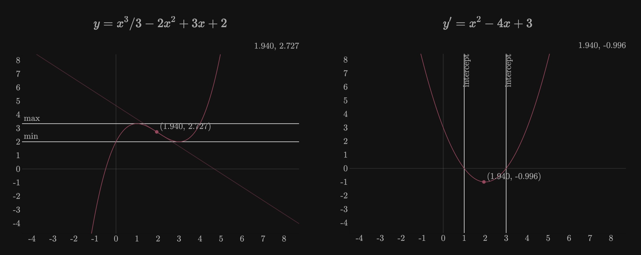
More generally if $y$ is a function of $x$ it seems that to find the maximum value of $y$ we must find $y^{'}$ and set it to 0

Let’s see an example, the following function has a maximum value of $3.333$ near $x = 1$ and a minimum value of $2$ near $x = 3$ , if we analyze the slope of the function near those points we will see that on the left of $x = 1$ the slope is positive and on the right of $x = 1$ the slope is negative, since we know that the derivative represents the slope of a function we can also expect that the derivative of this function near $x = 1$ will go from a positive value to a negative value intersecting the x-axis, if we analyze the slope near $x = 3$ will will see the same behavior with the slope but it’s going from a negative value to a positive one

y = x^{3} / 3 - 2 x^{2} + 3 x + 2

y^{'} = x^{2} - 4 x + 3

Now the problem reduces to finding the points where $y^{'} = 0$ in the derivative function, finding them will tell us exactly the maximum/minimum value of $y$ , finding the values of $x$ when $y^{'} = 0$

\begin{aligned} 0 & = x^{2} - 4 x + 3 \\ 0 & = (x - 1) (x - 3) \end{aligned}

And we see that:

y^{'} = 0 w h e n x = 1 a n d x = 3

The process didn’t actually find the maximum/minimum values since for $x > 3$ the function increases indefinitely, same goes when $x < 1$ but in this case the function decreases indefinitely, these values are called the relative maxima/minima because near $x = 3$ or $x = 1$ these points are the minimum/maximum that can be found

Applications of maxima/minima

refraction of light, we can build a function of time which relates the velocity/distance the light travels in different mediums, finding the derivative and making it equal to $0$ will find the relative minimum time needed to go from one point in the medium $a$ to a point in a medium $b$
finding the sides of the rectangle with the maximum perimeter

Newton-Raphson method

The slope of the tangent line of a function $f (x)$ at any derivable point is given by $m = f^{'} (x)$ , let $x_{1}$ be a derivable point then the slope of the tangent line at $x_{1}$ is $m_{1} = f^{'} (x_{1})$ , the Point–slope form of the tangent line whose slope is $f^{'} (x_{1})$ is

y - y_{1} = m_{1} (x - x_{1}) y - f (x_{1}) = f^{'} (x_{1}) \cdot (x - x_{1})

Newton find out that if we find the intercept of this tangent line with the $x$ -axis at some initial guess $x_{1}$ , the value found approaches one of the roots of $f (x)$ , i.e. when $f (x) = 0$ (obviously given that it has roots)

if $y = f (x) = 0$ then the equation of the line is

0 - f (x_{1}) = f^{'} (x_{1}) \cdot (x - x_{1})

Solving for $x$

\begin{matrix} (18) & x = x_{1} - \frac{f (x_{1})}{f^{'} (x_{1})} \end{matrix}

$x$ in the last equation is the abscissa of the next approximation of one of the roots of $x$ , if we run the algorithm above a few times with an acceptable initial guess then we’ll obtain a better approximation of one of the roots of $f (x)$

Finding the square root of a number

Let’s say that we want to find the square root of a number $n$ , this is equivalent to finding the solution to

x^{2} = n

The function to use is then

f (x) = x^{2} - n

whose derivative is

f^{'} (x) = 2 x

Substituting in $(18)$

\begin{aligned} x & = x_{1} - \frac{x_{1}^{2} - n}{2 x_{1}} \\ = x_{1} - \frac{x_{1}}{2} + \frac{n}{2 x_{1}} \\ = \frac{x_{1}}{2} + \frac{n}{2 x_{1}} \\ = \frac{1}{2} \cdot (x_{1} + \frac{n}{x_{1}}) \end{aligned}

double square_root(double n) {
  // initial guess
  double EPS = 1e-15;
  double x0 = 1;
  while (true) {
    double xi = (x0 + n / x0) / 2.0;
    if (abs(x0 - xi) < EPS) {
      break;
    }
    x0 = xi;
  }
  return x0;
}